Graphics Notes

Introduction

Graphics

Raster (bitmap) graphics have a fixed array of pixels with values, and a fixed resolution. Vector graphics are driven by display commands. It has a scalable resolution, which makes it ideal for typography and animation.

There are three main disciplines of graphics: modeling shape and appearance, animation, and rendering.

Images and Pixels

An image is a 2D grid of cells called pixels, where each pixel holds some set of values. A pixel (picture + element) is a unit with some kind of value. A pixel value can represent intensity (grayscale), color (RGB), opacity, or depth.

What are the advantages and disadvantages of floating-point vs. integer format?

Floating point takes a lot more storage than integer
24 bits is usually enough for the human eye
Floating point is usually used as the intermediate format for calculations

How do we store images in memory?

Array of structs (AoS), where each struct represents an RGB value
Struct of arrays (SoA), where each array represents a R, G, or B channel

Different memory organizations affect cache locality.

Vector Graphics

Vector Graphics Pipeline

To create a 2D vector graphic:

Define object geometry
Transform object (translate, rotate, scale)
Define "window" on the world
Render into raster graphics

In each of the steps of this pipeline, there are different coordinate systems:

Object geometry is defined in terms of object space
Objects are placed into world space
The window is defined in terms of view space
The rendered graphic is defined in terms of normalized device coordinates, which are resolution-specific
The application may only have a subregion of the OS window (viewport), so we might also need to transform into screen space

Why use multiple coordinate systems?

At higher levels of abstraction, we don't want to think about specific device coordinates to draw to. We also want to keep different layers modular, so we can modify each independently.

Scenes

Graphics applications typically represent scenes with a DAG which stores:

Objects
Attributes (color, texture)
Transformations

Scene graph of robot

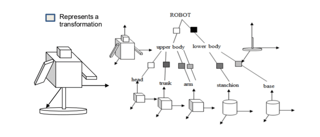
To get the cumulative transformation matrix of an object, simply walk the node up to the root.

Appendix

Vectors

A vector transforms a scalar into another scalar. Below, we transform the scalar $(x, y)$ by shifting it $a$ units right and $b$ units up.

(x, y) + \begin{bmatrix} a \\ b \end{bmatrix} = (x + a, y + b)

The dot product is an operation that takes in two vectors and produces a scalar:

\begin{bmatrix} a \\ b \end{bmatrix} \cdot \begin{bmatrix} c \\ d \end{bmatrix} = ac + bd

Geometric interpretations of the dot product:

$\begin{bmatrix} a \\ b \end{bmatrix}^2 = a^2 + b^2$ is the squared length of the vector
$\begin{bmatrix} a \\ b \end{bmatrix} \cdot \begin{bmatrix} c \\ d \end{bmatrix} = 0$ when the vectors are perpendicular
$v \cdot w = |v||w|\cos(\theta)$ , where $\theta$ is the angle between the arrows

The cross product is an operation that takes in two vectors and produces a vector that is mutually perpendicular to both vectors. By convention, the direction that $a \times b$ points in is determined by the right-hand rule.

a \times b = \begin{bmatrix} a_2b_3 - a_3b_2 \\ a_3b_1 - a_1b_3 \\ a_1b_2 - a_2b_1 \end{bmatrix}

Geometric interpretations of the cross-product:

$a \times b = |a||b| \sin(\theta)$
$a \times b$ also gives the area of the parallelogram with $a$ and $b$ as edges. Half of this area gives us the triangle with $a$ and $b$ as edges.

Matrices

The identity matrix is a matrix such that $MI = IM = M$ for all matrices $M$ . The 2x2 identity matrix is:

\begin{bmatrix} 1 & 0 \\ 0 & 1 \end{bmatrix}

If we have two matrices $M$ and $K$ such that $MK = I$ , then we say that $K$ is the inverse of $M$ . Not all matrices have an inverse. For a 2x2 matrix, we have:

\begin{bmatrix} a & b \\ c & d \end{bmatrix} \frac{1}{ad - bc} \begin{bmatrix} d & -c \\ -b & a \end{bmatrix} = I

Transformations

A transformation $T$ is a function that acts on space.

A linear transformation respects the property $T(a\hat{u} + b\hat{v}) = aT(\hat{u}) + bT(\hat{v})$
A matrix transformation is any transformation that can be written in terms of multiplying a matrix and a vector
Every linear transformation is a matrix transformation

Note that matrix transformations can compose. For example, applying $M$ then $K$ to vector $v$ is equivalent to $K(Mv) = (KM)v$ .

We can build matrix transformations using basis vectors. To find a matrix $M$ that sends:

\begin{equation*} e_1 = \begin{bmatrix} 1 \\ 0 \end{bmatrix} \text{to} \begin{bmatrix} x_1 \\ x_2 \end{bmatrix} \quad\mathrm{and}\quad e_2 = \begin{bmatrix} 0 \\ 1 \end{bmatrix} \text{to} \begin{bmatrix} y_1 \\ y_2 \end{bmatrix} \end{equation*}

We need to find a matrix that satisfies:

\begin{equation*} \begin{bmatrix} a & b \\ c & d\end{bmatrix}\begin{bmatrix} 1 \\ 0 \end{bmatrix} = \begin{bmatrix} x_1 \\ x_2 \end{bmatrix} \quad\mathrm{and}\quad \begin{bmatrix} a & b \\ c & d\end{bmatrix}\begin{bmatrix} 0 \\ 1 \end{bmatrix} = \begin{bmatrix} y_1 \\ y_2 \end{bmatrix} \end{equation*}

Arithmetically, this matrix is

\begin{bmatrix} x_1 & y_1 \\ x_2 & y_2\end{bmatrix}

To reverse the transformation, we can simply calculate the inverse of $M$ .

Thus, to send

\begin{equation*} \begin{bmatrix} a_1 \\ a_2 \end{bmatrix} \text{to} \begin{bmatrix} x_1 \\ x_2 \end{bmatrix} \quad\mathrm{and}\quad \begin{bmatrix} b_1 \\ b_2 \end{bmatrix} \text{to} \begin{bmatrix} y_1 \\ y_2 \end{bmatrix} \end{equation*}

We can simply calculate the matrix $M$ that sends

\begin{equation*} \begin{bmatrix} 1 \\ 0 \end{bmatrix} \text{to} \begin{bmatrix} a_1 \\ a_2 \end{bmatrix} \quad\mathrm{and}\quad \begin{bmatrix} 0 \\ 1 \end{bmatrix} \text{to} \begin{bmatrix} b_1 \\ b_2 \end{bmatrix} \end{equation*}

And the matrix $K$ that sends

\begin{equation*} \begin{bmatrix} 1 \\ 0 \end{bmatrix} \text{to} \begin{bmatrix} x_1 \\ x_2 \end{bmatrix} \quad\mathrm{and}\quad \begin{bmatrix} 0 \\ 1 \end{bmatrix} \text{to} \begin{bmatrix} y_1 \\ y_2 \end{bmatrix} \end{equation*}

And then calculate $K(M^{-1})$ .

Scale, Rotate, and Translate

Both scale and rotate are linear transformations and can be represented by matrix transformations.

To scale by $s_x$ in the x-axis and scale by $s_y$ in the y-axis, apply the matrix:
$\begin{bmatrix} s_x & 0 \\ 0 & s_y \\ \end{bmatrix}$
To rotate by $\theta$ counterclockwise, apply the matrix:
$\begin{bmatrix} \cos(\theta) & -\sin(\theta) \\ \sin(\theta) & \cos(\theta) \\ \end{bmatrix}$

Translation is not a linear transformation; it is an affine transformation. In order to represent it as a matrix transformation, we add a third coordinate $w$ .

$w$ is $1$ if the value is a scalars and $0$ if the value is a vector
$w$ does not affect subtraction of two scalars (which produces a vector), addition of a vector and a scalar (which produces a scalar), or dot product (which is mostly between two vectors)
$w$ also does not affect the linearity of scaling and rotation $\begin{equation*} \begin{bmatrix} a & b \\ c & d\end{bmatrix} \quad\rightarrow\quad \begin{bmatrix} a & b & 0 \\ c & d & 0 \\ 0 & 0 & 1\end{bmatrix} \end{equation*}$

To translate $dx$ in the x-axis and $dy$ in the y-axis, apply the matrix:

\begin{bmatrix} 1 & 0 & dx \\ 0 & 1 & dy \\ 0 & 0 & 1\end{bmatrix}

Algorithmically, this works to out be:

\begin{bmatrix} 1 & 0 & dx \\ 0 & 1 & dy \\ 0 & 0 & 1\end{bmatrix} \begin{bmatrix} x \\ y \\ 1\end{bmatrix} = \begin{bmatrix} x + dx \\ y + dy \\ w\end{bmatrix}

Non-Axis Aligned 3D Rotation

Scaling and translation in 3D is similar to that in 2D. Rotations are more complicated because we can now rotate around an arbitrary axis. There are several ways to do this: Euler angles, axis-angles, and quaternions.

Euler angles are a composition of rotations around the x, y, and z axes. One problem with Euler angles is that they don't trace the shortest rotational path because rotation composition doesn't commute. To fix that, we can linearly interpolate each angle independently with some correction factor. However, this does not get an even angular velocity. Finally, when two rotation axes align, we lose a degree of freedom, causing sudden jumps (gimbal lock).

Axis-angle rotations involve decomposing a point $x$ into two parts relative to the axis $r$ :

$x_\parallel$ is the part parallel to $r$ ; rotation does not change it
$x_\perp$ is the part perpendicular to $r$ ; it rotates like a 2D point in a plain perpendicular to $r$

To calculate it, we need:

x' = x_\parallel + x\vdash\sin(\theta) + x_\perp\cos(\theta)

Which can be expanded to:

x' = (\hat{r}(\hat{r} \cdot x)) + (\hat{r} \times x)\sin(\theta) + (-\hat{r} \times (\hat{r} \times x))\cos(\theta)

The formula for the cross product can be represented as a matrix, so this entire equation can be rewritten in matrix form. Unfortunately, axis-angle rotations also do not sweep the shortest path between two points.

Quaternions are the only rotation method that can correctly do linear interpolation. A quaternion represents a rotation as a point on the surface of a 4D hypersphere. Because we are moving along the sphere, we get shortest path and constant angular velocity.

References: Visualizing quaternions