Arrays
An array is a contiguous block of memory used to represent sequences. In terms of time complexity:
- Retrieving and updating an element takes O(1) time
- Inserting into an array takes O(1) time, amortized
- Deleting an element involves moving all successive elements one over, taking O(n - i) time
A subarray is a contiguous part of an array. Techniques for solving such problems include:
A subsequence is a sequence derived from an array by deleting elements without changing the order of the remaining elements. Techniques for solving such problems include:
It is also often the case that we need to have a sorted array. While most programming languages have a built-in sorting method, it never hurts to know a few sorting algorithms. Sorted arrays are particularly helpful for search problems, which can usually be handled by binary search.
Finally, there are also multidimensional array problems.
Two Pointer
Two pointer is a technique to find valid subarrays. The basic idea is to keep two pointers, l and r, and move l or r depending on some condition.
def f(arr):
    l, r = 0, len(arr) - 1
    while l < r:
        if cond:
            l += 1
        else:
            r -= 1
    return l
Problems: 3Sum, Container With Most Water and Trapping Rainwater
Sliding Window
Sliding window is a technique used to find valid subarrays.
Time complexity: There are subarrays, but a sliding window runs in O(n).
def f(arr):
    output, l, curr = 0, 0
    for r in range(len(arr)):
        curr += arr[r]
        while curr > k:
            curr -= arr[l]
            l += 1
        output = max(output, r - l + 1)
    return output
Prefix and Suffix Array
Prefix arrays store the running total of elements from the start of an array up to each index. It is used to answer range queries in constant time.
def prefix_sum(arr):
    prefix = [arr[0]]
    for i in range(1, len(arr)):
        prefix.append(prefix[i-1] + arr[i])
    return prefix
Problems: Product of an Array Except Self
Kadane's Algorithm
Kadane's algorithm is used to find the maximum sum of a contiguous subarray. At each step, either start a new subarray at n, or extend the previous subarray with curr_sum + n.
def f(arr):
    curr_sum = 0
    best_sum = float('-inf')
    for n in arr:
        curr_sum = max(n, curr_sum + n)
        best_sum = max(best_sum, curr_sum)
    return best_sum
Problems: Maximum Subarray, Maximum Product Subarray
Sorting Algorithms
Sorting algorithms are used to sort an array.
Time complexity: O(n log n)
Merge sort recursively breaks the array into left and right subarrays, sorts them, and merges the sorted lists. In the base case, the list is length 0 or 1 and is considered sorted.
def merge_sort(arr):
    if len(arr) <= 1:
        return arr
    mid = len(arr) // 2
    left = merge_sort(arr[:mid])
    right = merge_sort(arr[mid:])
    return merge(left, right)

def merge(left, right):
    output = []
    i = j = 0
    while i < len(left) and j < len(right):
        if left[i] <= right[j]:
            output.append(left[i])
            i += 1
        else:
            output.append(right[j])
            j += 1
    output.extend(left[i:])
    output.extend(right[j:])
    return output
Binary Search
Binary search is used to find a specific element in a monotonic array. An array is monotonic if it is sorted, or if we can define some kind of condition that switches from true to false along the array.
Time complexity: O(log n)
The most basic binary search is:
def binary_search(arr, target) -> int:
    l, r = 0, n
    while l <= r:
        m = (l + r) // 2
        if arr[m] == target:
            return m
        elif arr[m] > arr[l]:
            l = m + 1
        else:
            r = m - 1
    return -1
A more generalized template is:
def binary_search(arr) -> int:
    def cond(i) -> bool:
        pass

    l, r = 0, n
    while l < r:
        m = (l + r) // 2
        if cond(m):
            r = m
        else:
            l = m + 1
    return l
This finds the first element that appears True after a sequence of False.
Problems: Search a 2D Matrix.
References: Powerful Ultimate Binary Search Template
Multidimensional Array
In a multidimensional array, it is important to pay attention to dimensionality. Visually, the first index generally represents the row, and the second index represents the column. Thus, arr[i][j] refers to the element in the ith row and jth column.
Note that some multidimensional array problems are actually graph problems in disguise.
Problems: Spiral Matrix, Rotate Image
Linked Lists
A linked list is a sequence where each element has a pointer to the next element in the list.
In terms of time complexity:
- Searching for a node takes O(n) time
- Inserting and deleting a node takes O(1) time
Dummy Nodes
Use a dummy node to avoid checking for empty lists, in cases where the head of the list needs to be removed or modified.
Problems: Reverse Linked List), Merge Two Sorted Lists, and Remove Linked List Elements.
Reverse Linked List
Reverse a linked list whenever you need to traverse the list in the opposite direction.
def reverse(head):
    prev = None
    curr = head

    while curr:
        temp = curr.next
        curr.next = prev
        prev = curr
        curr = temp

    return prev
Problems: Palindrome Linked List, Reorder List,
Fast and Slow Pointers
Fast and slow pointers are useful for finding elements or identifying cycles. In particular, they can be used to:
- Detect cycles in a linked list
- Find where a cycle begins in a linked list
- Find the middle of a linked list
The basic idea is that the fast pointer moves forward by two units, while the slow pointer moves forward by one unit. If there is a cycle, fast will eventually circle around and pass slow.
def has_cycle(head):
    slow, fast = head, head
    while fast and fast.next:
        slow = slow.next
        fast = fast.next.next
        if fast == slow:
            return True
    return False
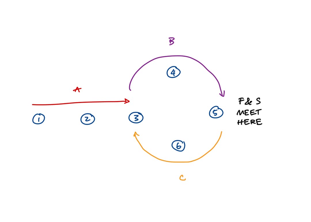
We can also use this idea to find where the cycle begins. At the point when slow and fast meet, we have A + B = A + B + C + B. We also know that slow is half the speed of fast, so 2(A + B) = A + B + C + B. Simplifying, we get A = C.
Problems: Reorder List, Delete the Middle Node of a Linked List
Stacks and Queues
A stack supports two operations: push and pop. Elements are pushed and popped in a last-in, first-out (LIFO) order. If implemented with an array or linked list, all operations are O(1).
Problems: Implement a Stack with Max API, Evaluate Reverse Polish Notation, Valid Parentheses
A queue supports two operations: enqueue and dequeue. Elements are added (enqueued) and removed (dequeued) in first-in, first-out (FIFO) order. A dequeue, or a double-ended queue, is a doubly linked list in which all insertions and deletions are from one of the two ends of the list.
Queues can be implemented using linked lists, arrays, and even stacks. The main idea behind the stack implementation is to use one stack for enqueues, and another stack for dequeues.
As you might have noticed, stacks and queues are ordered by time of insertion. They are different from priority queues (also know as Heaps), which order by the value of the element.
Trees
A tree is a directed graph where each node has exactly one parent, except for the root node.
A tree can be constructed by having each parent store pointers to their child nodes.
class Node:
    def __init__(self, value):
        self.value = value
        self.children = []
Tree Traversal
There are multiple ways to traverse a tree. They can be categorized by whether they are depth-first (DFS) or breadth-first (BFS). There are three variants of DFS: pre-order (node-left-right), post-order (left-right-node), and in-order (left-node-right).
DFS needs a stack, so it is usually implemented recursively to take advantage of the call stack. However, it can also be implemented iteratively.
# DFS, pre-order, recursive
def traverse(node):
    if node is None:
        return
    visit(node)
    traverse(node.left)
    traverse(node.right)
# DFS, pre-order, iterative
def traverse(root):
    if root is None:
        return
    stack = [root]
    while len(stack) > 0:
        node = stack.pop()
        if node is None:
            continue
        visit(node)
        # note that right is pushed first
        # so that left is processed first
        if node.right is not None:
            stack.push(node.right)
        if node.left is not None:
            stack.push(node.left)
BFS needs a queue to keep track of nodes at the current level, so it is usually implemented iteratively.
# BFS, iterative
def traverse(root):
    curr = [root]
    while curr:
        nxt = []
        for node in curr:
            if node is not None:
                for child in node.children:
                    nxt.append(child)
        curr = nxt
Tries
A trie (also known a prefix tree) is a tree data structure used to efficiently store and retrieve keys in a set of strings.
class PrefixTree:
    def __init__(self):
        self.children = {}
        self.terminated = False

    def insert(self, word: str) -> None:
        if len(word) == 0:
            self.terminated = True
            return

        c = word[0]
        if c not in self.children:
            self.children[c] = PrefixTree()
        self.children[c].insert(word[1:])

    def search(self, word: str) -> bool:
        if len(word) == 0:
            return self.terminated
        c = word[0]
        if c not in self.children:
            return False
        return self.children[c].search(word[1:])

    def startsWith(self, prefix: str) -> bool:
        if len(prefix) == 0:
            return True
        c = prefix[0]
        if c not in self.children:
            return False
        return self.children[c].startsWith(prefix[1:])
Binary Trees
A binary tree is a type of tree where nodes can have at most two children.
Complete Binary Trees
A complete binary tree is completely filled on every level from left to right.
Complete binary trees are often implemented with arrays for efficiency. Let the root node be index 0. For a given node at index i:
- Its left child is at index
2 * i + 1 - Its right child is at index
2 * i + 2 - Its parent is at index
floor((i - 1) / 2)
Complete binary trees are used in binary heaps and segment trees.
Segment Trees
A segment tree is used for range queries and updates.
Time complexity: It can achieve both in O(log n) time. This is better than simple loops, which take O(n) time for querying, and prefix sums, which take O(n) time for updates.
tree = [0] * (2 * n) # n is the len of the array

def build(arr):
    # arr is at the bottom of the tree
    # from n to 2n-1
    for i in range(n):
        tree[i + n] = arr[i]
    # parents start at n-1 and before 0
    # the left child is at 2i and the right child is at 2i + 1
    for i in range(n - 1, 0, -1):
        tree[i] = tree[i << 1] + tree[i << 1 | 1]

# [l, r)
def query(l, r):
    output = 0
    l += n # index of l in tree
    r += n # index of r in tree
    while l < r:
        # if l is a right child node, take it
        if l & 1:
            output += tree[l]
            l += 1
        # if r is a right child node, take the left child
        # because of exclusive or
        if r & 1:
            r -= 1
            output += tree[r]
        # get the next parent
        l >>= 1
        r >>= 1
    return output

def update(i, val):
    i += n # index of val in tree
    tree[i] = val
    while i > 1:
        # parent is the sum of its children
        tree[i >> 1] = tree[i] + tree[i^1]
        i >>= 1
Problems: Block Placement Queries.
References: [1].
Heaps
A heap is a tree-based data structure that satisfies the heap property, which states that a parent node should be less than (or greater than) its children nodes. Use a heap when all you care about is the largest or (or smallest) elements, and you do not need to support any operations for arbitrary elements.
A heap can be implemented using a binary tree, in which case it is called a binary heap.
- In
push, instantiate the element to the bottom left of the binary tree. While the element is smaller than its parent, swap it. - In
pop, take out the root and replace it with the node at the bottom left of the tree. While the new root is larger than either of its children, swap with the smaller child.
In terms of time complexity, it supports:
- O(log n) insertions
- O(1) lookup for max element
- O(log n) deletion of the max element
Binary Search Trees
A binary search tree (BST) is a binary tree which enforcs a global left-right order. For every node, all values in the left subtree are smaller than the node, and all values in the right subtree are larger than the node. An in-order traversal of a BST yields a fully sorted list.
In terms of time complexity:
- Finding the min and max elements is O(log n)
- Lookup, deletion, and search is also O(log n)
Problems: Lowest Common Ancestor of a Binary Search Tree,
Hashmaps
A hashmap stores information in key-value pairs. It uses a hash function to turn a key into an index, where the value is stored.
In terms of time complexity, it supports:
- O(1) insertion
- O(1) lookup
Because keys are hashed, there is no ordering in a hashmap. It's very important to make sure that keys hash to the same value, so one should avoid having mutable keys.
If two keys map to the same location, there will be a collision, which can be handled by:
- Separate chaining
- Open addressing via linear probing
Graphs
A graph is a data structure with a set of nodes connected by edges.
Shortest Path
To find the shortest path from a source node k to all other nodes in a weighted graph, we can use Dijkstra's algorithm or the Bellman-Ford algorithm.
Dijkstra's algorithm
- Create a set of all unvisited nodes
- Assign every node a distance from the starting node. For the starting node, it is 0, and for all other nodes, it is ∞
- Maintain a priority queue ordered by distance, initially containing only the starting node with distance 0
- Pop the node with the smallest distance from the priority queue. If it has already been visited, skip it; otherwise mark it as visited and remove it from the set of unvisited nodes
- For each unvisited neighbor, if the distance to the current node plus the edge weight to the neighbor is less than the neighbor's current distance, update the neighbor's distance and push it into the priority queue
- Repeat until the priority queue is empty. Every node now holds its shortest distance from the starting node
Dijkstra's Algorithm
Bellman-Ford algorithm
- Assign every node a distance from the starting node. For the starting node, it is 0, and for all other nodes, it is ∞
- Repeat the following step
n - 1times (once for each of thennodes minus the starting node): for every edgeu -> vwith weightw, if the distance toupluswis less than the distance tov, update the distance tov. This is called relaxation - After the
n - 1passes, check all edges once more. If any relaxation is still possible, the graph contains a negative-weight cycle, and a shortest path does not exist
Bellman-Ford works on graphs with negative edge weights (unlike Dijkstra's), at the cost of running in time instead of . The n - 1 passes are enough because any acyclic shortest path uses at most n - 1 edges.
Bellman-Ford Algorithm
Topological Sort
Topological sort is used to find an ordering on a directed acyclic graph. Note that the ordering may not be unique, and there is no ordering if there is a cycle.
Kahn's algorithm
- Find all free nodes with no dependencies
- Whenever a free node is added to the ordering, decrement the degree of its neighboring nodes.
- If the length of the ordering is less than the number of nodes in the DAG, then there is at least one cycle.
Kahn's Algorithm
Depth-first search
- While there are unvisited nodes, choose a random node and perform DFS on it.
- Mark each visited node in the seen list, then keep recursing into its unvisited neighbors.
- When you reach a node with no unvisited neighbors, push it into the ordering and backtrack.
- If you ever reach a node that's seen but not yet in the ordering, there is a cycle.
DFS Topological Sort
References: Kahn's Algorithm and Topological Sort with DFS.
Union Find
Union find is used to keep track of disjoint sets. To determine whether a and b are in the same sets, simply check whether find(a) == find(b).
Union find is constructed by maintaining a representative element ("parent") for the entire set.
uniontakes two elements and combines their sets by making one element the parent of the otherfindtakes an element and returns the topmost parent
parent = list(range(n))

def find(i):
    if parent[i] == i:
        return i
    return find(parent[i])

def union(a, b):
    pa, pb = find(a), find(b)
    parent[pa] = pb
find can be optimized with path compression, which flattens the structure of the tree whenever find is called. This means that every node points directly to the topmost parent, speeding up future find operations.
union can be optimized with rank-ordering, which keeps track of the maximum height of the trees. When two trees are combined, the tree with a lower height is made a child of the tree with a higher height. This keeps the overall structure more balanced and prevents long chains of nodes, which would slow down find operations. Only when the heights of the trees are equal could the height increase.
parent = list(range(n))
rank = [0] * n

def find(i):
    if parent[i] == i:
        return i
    parent[i] = find(parent[i])
    return parent[i]

def union(a, b):
    pa, pb = find(a), find(b)
    if pa == pb:
        return
    if rank[pa] > rank[pb]:
        parent[pb] = pa
    elif rank[pa] < rank[pb]:
        parent[pa] = pb
    else:
        parent[pa] = pb
        rank[pb] += 1
Dynamic Programming
Dynamic programming is used for problems where future decisions depend on earlier decisions. This may involve looking for the optimum value or the number of ways to do something.
One way to do dynamic programming is with top-down memoization.
memo = {}
def fib(n):
    if n <mark> 0 or i </mark> 1:
        return n
    if n not in memo:
        memo[n] = f(n - 1) + f(n - 2)
    return memo[n]
Another way to do dynamic programming is from the bottom-up. Start with base cases and iteratively build up to the solution in order.
def fib(n):
    if n == 0:
        return 0
    prev, curr = 0, 1
    for i in range(2, n):
        prev, curr = curr, prev + curr
    return curr
1D Problems: Best Time to Buy and Sell Stock, Climbing Stairs, Coin Change
2D Problems: Best Time to Buy and Sell Stock with Cooldown, Coin Change II, Target Sum, Longest Common Subsequence
Backtracking
Backtracking is used to solve constraint satisfaction problems (CSP) where partial candidate solutions which can be checked relatively quickly.
The general idea is to incrementally build candidates to the solution. Abandon a candidate ("backtrack") as soon as you determine that the candidate cannot lead to a valid solution.
def f():
    output = []  # All possible solutions
    partial = [] # Current partial solution

    def backtrack():
        nonlocal output, partial

        # Base case
        if is_solution(partial):
            output.append(partial[:]) # Need to copy the list
            return

        # Pruning
        if invalid(partial):
            return

        # Try every candidate
        for c in candidates:
            partial.append(c) # Add to the partial
            backtrack(i + 1)
            partial.pop()     # Remove from the partial

    backtrack()
    return output
Problems: Permutations and Combinations.